

Have you ever needed to change out some data in a Cell in Excel but wanted to keep the original value intact (meaning you can’t do a bulk search and replace)? Then Excel’s SUBSTITUTE function might be the exact function you need. Here’s how to use it.
First off, a few notes about the SUBSTITUTE function:
- It’s case sensitive, so be aware of that.
- You can’t use it for wildcard-type searches (you’d still have to use search and replace for that).
- You can use this for hard-coded values or cell references.
To start changing things, open up an Excel spreadsheet and click on the cell you want to display your substitution:
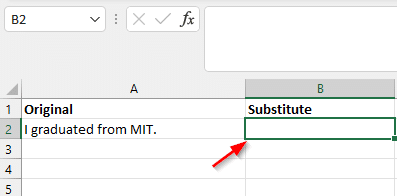
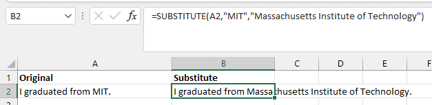
In this example, we’re going to substitute MIT with Massachusetts Institute of Technology. So we would use the following formula to make that change:
=SUBSTITUTE(A2,"MIT","Massachusetts Institute of Technology")
Basically, that formula looks at the data in cell A2, looks to see if anything says “MIT” and changes it and outputs the substitution in the column:
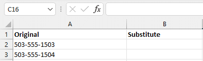
 The above example would change all instances of “MIT” to the longer value, but you can actually limit it to just the first one it finds. For example, some of us older Oregonians remember when a lot of the state’s geographic area switched from the 503 area code to 541. If you had a lot of phone numbers in your database with 503 in them, you’d want to update them to 541 without messing with the other numbers in the phone number. In this case, here’s your original data:
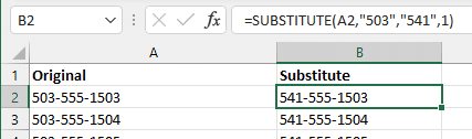
In this case, you could use this formula:
=SUBSTITUTE(A2,"503","541",1)
In this case, the “1” at the end of the formula limits the substitution to just the first one it finds:
 What’s your favorite Excel function? Let us know in the comments below!